From biological inspiration to the mathematical “engine” of backpropagation.
This week, I began the first of a three-part journey into the core of modern AI: Neural Networks and Deep Learning. While I’ve spent weeks on individual algorithms like SVMs and Decision Trees, this module marks the transition into how computers learn complex patterns by mimicking the human brain.
Here are the foundational building blocks I explored:
1. The Artificial Neuron (The Perceptron)
Artificial neurons are simplified mathematical models inspired by biological cells. While a biological neuron uses dendrites and axons to transmit signals, an artificial one uses math:
- Inputs (xi): Raw data or signals from other neurons.
- Weights (wi): “Importance scores” that tell the neuron how much attention to give each input.
- Bias (b): An adjustment term that helps the neuron shift its response to better fit the data.
- Activation Function (Φ): This introduces nonlinearity, allowing the neuron to model complex patterns.
The standard formula for a neuron’s output is:
Output = Φ(w1.x1 + w2.x2 + … + wn.xn + b)
2. The Universal Approximation Theorem
A major highlight of this module was learning about George Cybenko’s 1989 proof. He showed that a simple neural network with just one hidden layer and enough neurons can approximate any continuous function. This “Universal Approximation Theorem” proved that neural networks are incredibly powerful, even with simple architectures.
3. Activation Functions: Sigmoid vs. ReLU
I learned that the choice of activation function determines how the network “thinks”:
- Sigmoid: An S-shaped curve that maps inputs to a range between 0 and 1—perfect for predicting probabilities.
- ReLU (Rectified Linear Unit): The modern standard (r(x) = max(0, x)). It is computationally efficient and helps deep networks learn much faster.
- Leaky ReLU: A variation that prevents neurons from “dying” (becoming inactive) by allowing a tiny signal through for negative inputs.
4. Learning through Gradient Descent
To learn the right weights, the network must minimize its Loss Function (the measure of its errors). It does this through Gradient Descent, which iteratively adjusts parameters in the opposite direction of the error’s “slope”.
| Type | Description | Pros | Cons |
| Batch (BGD) | Uses the entire dataset for every update. | Stable and accurate. | Very slow on large data. |
| Stochastic (SGD) | Updates parameters after every single example. | Very fast; helps escape local minima. | Noisy and erratic convergence. |
| Mini-Batch | Uses small groups (16–256 samples). | Balanced speed and stability. | Requires tuning batch size. |
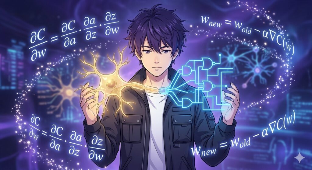
5. Backpropagation: The Engine of Learning
The most important algorithm in deep learning is Backpropagation. It uses the Chain Rule of calculus to trace errors from the output layer backward through the hidden layers. This process “unravels” the error layer by layer, telling every single weight in the network exactly how much it needs to change to improve the next prediction.
Conclusion
Module 15 laid the groundwork for everything else to come. By combining simple linear operations with nonlinear activations and optimizing them with backpropagation, we can build systems that can recognize faces, translate languages, and drive cars.
Next up: Deep learning frameworks like PyTorch and real-world application strategies!