
Learning from similarity, the “Curse of Dimensionality,” and why you should always scale your data.

This week marks the beginning of Phase 2 of my Machine Learning Professional Certificate! We are moving beyond general principles and diving into specific algorithms. Module 8 focuses entirely on Nearest Neighbour Methods, specifically the k-Nearest Neighbors (k-NN) algorithm.
k-NN is built on a very intuitive underlying bias: similar inputs lead to similar outputs.
Here is a breakdown of the fascinating mechanics behind this algorithm:
1. Learning in the Dark: The k-NN Concept
The module used a great analogy: imagine eating at a “dark dining” restaurant. To figure out what you’re eating, you compare its crunchiness and sweetness to past experiences. If it’s sweet and juicy, it’s probably fruit.
k-NN does exactly this. To classify a new data point, it plots it on a graph, finds the k closest past examples (neighbors), and takes a majority vote . If we are doing regression (predicting a number like a house price), it simply takes the average—or a distance-weighted average—of those neighbors.
2. How Do We Measure “Close”?
For the algorithm to find the “nearest” neighbor, we have to define what distance means mathematically. I learned several ways to do this:
- Euclidean Distance: The “bird’s eye” view, measuring a direct straight line between two points.
- Manhattan Distance: The “taxicab” view, measuring the distance in right angles, as if navigating city blocks.
- Cosine Distance: Measures the angle/alignment between two vectors rather than their absolute position—hugely popular in text analysis.
3. The Golden Rule: Always Scale Your Data
If you measure “crunchiness” on a scale of 1 to 10, but measure “spiciness” on a scale of 1 to 15 million (like Scoville units), the distance calculation will be completely dominated by spiciness . The model will go blind to every other feature.
To fix this, we have to scale our data using Min-Max Normalization (scaling to a 0-1 range) or Z-Score Standardization (scaling based on mean and standard deviation).
4. Finding the Optimal k (Bias vs. Variance)
Choosing the number of neighbors (k) is the ultimate test of the bias-variance trade-off:
- Small k (e.g., k=1): The boundary is highly flexible and “wiggly.” It captures intricate patterns but is highly prone to overfitting noise.
- Large k (e.g., k=99): The boundary is smooth and stable. It resists noise but is prone to underfitting and missing the true pattern.
- You can’t just use your training data to pick k, because k=1 will always win (a point is always identical to itself). You must use a validation set to find the sweet spot.
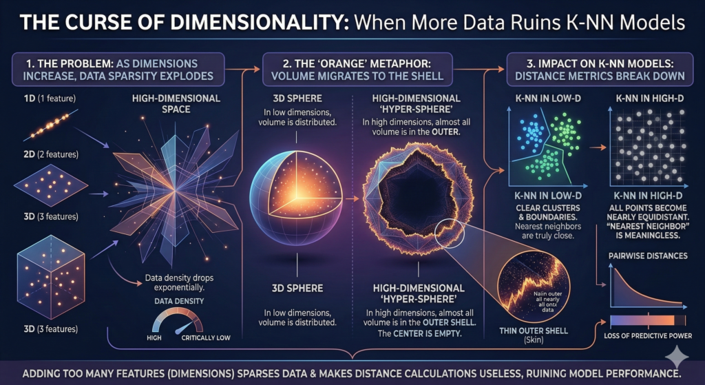
5. The “Curse of Dimensionality”
This was the most mind-bending concept. As you add more features (dimensions) to your dataset, standard distance metrics start to break down . In high-dimensional space, the “nearest” points are actually very far away.
The course compared it to an orange: as dimensions grow, almost all the volume of the space migrates to the outer shell (the skin), leaving the center empty . This means adding too many features can actually ruin a k-NN model!
Conclusion
k-NN is wonderfully simple and versatile—it’s even used to analyze the audio features of Beatles songs to figure out if John Lennon or Paul McCartney wrote them ! But it has limits: it’s a “lazy learner” that is slow to classify, it requires heavy data preprocessing, and it suffers greatly in high dimensions.
Next up, I’ll be looking into Decision Trees!